VAC - Advanced Excel Techniques - Conditional Formatting

 In this post, you can know how to work with Conditional Formatting

Conditional Formatting

·         Conditional formatting is used to change the appearance of cells in a range based on your specified conditions.

·         The conditions are rules based on specified numerical values or matching text.

First create a table of data as shown in the following

Apply the formula for total and Average

For total in the Cell L5    type the following

=I5+J5+k5

For average in the cell M5 type the following

= L5/3.0

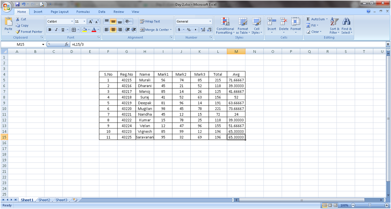
Now the total and Average is calculated.

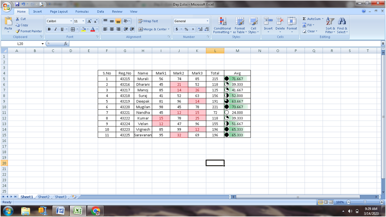
Now you can format the Column M via color scale based on the values.

Step 1 : Select the value M5 to M15

Step 2 : Click conditional Formatting in the Style (group) of Home Toolbar.

Select Color Scales and select the color pattern you want.

 

Similarly, you can apply the following  

Highlight the cell, if the cell value is greater than or lesser than the value mentioned.

Marks are selected from I5 to K15.

Select the Highlight Cells Rules, Select Less than.   (The objective is to highlight the marks which are less than 40).

Now apply Databar.

Select the Average – M5 to M15 and

Select the Conditional Formatting and Click Data Bar

Select the Color and show the data bar appeared in each cell.

Each value has the bar based on the value.

 

Try ICON SETS

 

Based on the cell Value the Icon will be appeared in front of the value.

Creating New Rule:

1.       Select Total Column

2.       Select New Rule

3.       Click New Rule

 

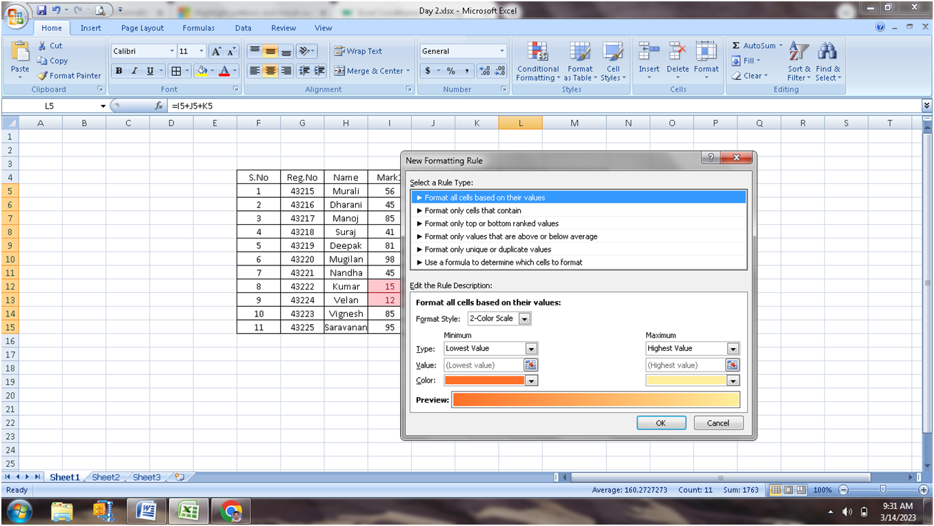
For the total between 100 to 200 is to highlighted with Red Border – Yellow background and text in Blue Color.

 

Click format and select the color needed.

 

 

Click OK to apply the format

 

 

 Clear the Rules:

 Formatting applied in the sheet shall be cleared either as whole for the entire sheet or clear for the selected cells.

 

 

Click “clear rules from Selected Cells”

To View all the Formatting rules applied

Click Manage Rule in the Conditional Formatting Submenu.

Show formatting rules for the “This Worksheet”

From here you can create new, modify the existing and delete the rules.

Kindly practice the same and get expert in formatting the data.